![]()
and
![]()
![]()
and
![]()
The Difference between Scorpion and Formiga
Formiga is a compilation of the tools used to calculate the frequency of 3D contacts as well as frequency of occurrence of the amino acids at the interface formed by facing chains in a given PDB format file(s). At the same time, those tools allow to the user to visualize results in graphically convenient and easy to interpret way. The user provides information as requested on the entry page of FORMIGA. In case of calculating the frequency of occurrence of the amino acids at the interface, for example, it is required that the user provides following information: a) names of proteins (PDB file names) and b) chain names that will belong to facing subunits and that should be used during calculation. The program defines the interface between given subunits. The program operates with two subunits that will form the interface. Those two subunits can contain protein chains and those are grouped in a way that the user indicates. Once the interface and its closest vicinity is identified (by calculating lost surface area upon complex formation between two subunits), the program will count amino acids in that defined region and present them in graphically convenient way. In case of 3D contacts, the user should inform the radius of the sphere within which the contacts will be counted. In addition, the user should choose the central residue for which the contacts will be identified and counted, as well as the atom from which the distances will be counted (Alpha Carbon or Last Heavy Atom in the amino acid side chain). The user can also choose the secondary structure element to which the central residue belongs and from which the contacts will be counted.
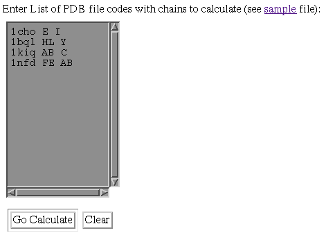
In this example, we have chosen to elaborate data on following
PDB files: 1cho.pdb 1bql.pdb 1kiq.pdb and 1nfd.pdb
The idea is to calculate 3D contacts and frequency of aminoacid occurrence in
an ensemble of similar proteins (this case is formed from arbitrary PDB files,
but the user is encouraged to try the ensemble of serine proteases or alpha
amylases or any other protein family of interest). Following 4 letter PDB code
is the space and then the single letter code(s) indicating the chain(s) that
form the FIRST subunit. After the space, the user enters the single letter code(s)
of the chain(s) that would form the SECOND subunit. So in this example, 1cho.pdb
will be processed in such way so that the interface will be formed between chain
E and chain I. For 1bql.pdb, the interface will be formed between the FIRST
subunit formed by H and L chains and the second subunit formed by the Y chain.
In pdb file 1kiq.pdb, the interface will be formed between the FIRST subunit
(containing the chain A and B) and the SECOND subunit containing only the C
chain. In case of 1nfd.pdb, the FIRST subunit is formed by the F and the E chain,
while the SECOND subunit is formed by the A and B chain.
The user will receive from FORMIGA the data on each PDB file as well as on the
TOTAL (sum of frequencies) in the ensemble of PDB files indicated.
After choosing properly PDB files for 3D contacts and amino acid frequency calculation, Formiga will present the window as shown bellow:
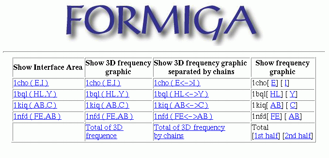
To show calculated data on 3D contacts for specific PDB file, the user should
click on that PDB item in the column: "Show 3D frequency graphic".
If the user wants to see data for all chosen PDB files, than the user should
click on "Total of 3D frequency".
However, before the actual data are shown, the user will be presented with the
window as this bellow:
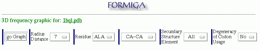
In this window, the user can choose appropriate parameters for the calculation of the 3D contacts. Radius Distance option will specify the maximum distance for the 3D contacts. The option Residue will fix the base residue from which the 3D contacts will be calculated. In another words, 3D contacts will be calculated only for the pairs where at least one amino acid is the base residue. The third option is for the choice of the atom from/to which the distances will be calculated: (CA-CA and LHA-LHA); CA is the Carbon Alpha atom e LHA is the Last Heavy Atom in the amino acid side chain. The option Secondary Structure Element will indicate to the program the restriction in terms of the conformation where the base residue should be located so that the calculation will take into account the encountered contact or not. The last option Degeneracy of Codon Usage is not available yet.
Once all options are chosen, it is necessary to click on go graph and the window as this one bellow will be generated.
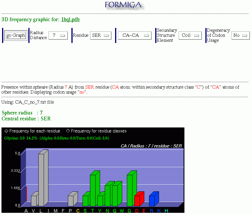
In this example, "Glycine: 3.0" indicates that there are 3 contacts in 3D between glicine and the base residue (serine, in this example) in the 1bql.pdb file. "14.2%" indicates that those 3 contacts represent 14,2% of total contacts in 3D and , "||Alpha: 0.0 |Beta: 0.0 | Turn: 0.0 | Coil: 3.0 ||" indicates that 3 glycines that make the contact with the base residue, 0 are in the alpha helix conformation, 0 are in the beta conformation, 0 are in the turn conformation and 3 are within coil conformation. Similar information is available for any of the 20 amino acids. The user should "walk"the mouse above the graphical bars and information will appear on the status area. In case that the user did NOT choose the Secondary Structure Element, that is, indicating ALL secondary structure elements, FORMIGA will present non differentiated (cumulative) number, representing the frequency for all elements of SS. The user still has the option to click on the Frequency for residue classes and the graph will assume the form which sums hydrophobic, charged, polar residues and the glicine in cumulative graphic bars.
The procedure in this case is similar to the two above cases. After selecting
the group of PDB files (see How to choose PDB files to be
processed?), the user should go to the column "Show frequency graphic" and
click on the FIRST or the SECOND subunit. In case that the user needs to calculate
the frequency of occurrence for the amino acids for ALL chosen PDB files, the
user should click on "1st half", to calculate the frequency in the FIRST subunit,
or click on "2nd half", to calculate the frequency in the SECOND subunit.
The result is presented in the histogram
as shown bellow:
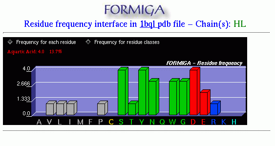
In this example, "Aspartic Acid: 4.0" indicates that there are 4 aspartic acids in subunit HL of the PDB file 1bql.pdb, and "13.7%" indicates that this number represents 13.7% of the total number of residues in this subunit. Positioning the mouse above any of the graphic bars, FORMIGA will show exact quantity of amino acid residue in this particular subunit. The option "Frequency for residue classes" will show reduced graph, grouping amino acids in their respective classes.
Introdução
Diferenças Entre Scorpion e Formiga
Formiga é um conjunto
de ferramentas utilizado para fazer o cálculo da frequência de
contatos 3D e da frequência de resíduos na região de
interface de arquivos pdb, bem como proporcionar uma visualização
gráfica dos resultados obtidos. O cálculo é feito com base
em informações obtidas do usuário que deverá
fornecê-las conforme requisitado pelo programa. No caso da
frequência de resíduos, por exemplo, é necessário
que o usuário informe os nomes das proteínas (pdb's) e as
regiões (subunidades) dentro de cada proteína que deverão
ser consideradas nos cálculos. O programa então define uma
região de interface, que é simplesmente a região envolvendo
a fronteira entre essas subunidades e suas imediações, e conta os
resíduos presentes nessa região, exibindo um gráfico com o
resultado. No caso da frequência de contatos 3D, além dos nomes das
proteínas e das subunidades, o usuário deve informar o raio de
contato, o resíduo central da esfera de contato, a
conformação desse resíduo e também o átomo
que será utilizado no cálculo das distâncias
(Carbono Alpha, etc). O usuário deverá ainda informar em quais das
subunidades definidas (primeira, segunda ou ambas) o cálculo será
feito, ou se apenas a interface entre uma subunidade e outra deve ser
considerada.
Conteúdo
Escolhendo
o Conjunto de Arquivos Pdb a Serem Processados
O usuário deverá entrar com o nome de cada arquivo pdb na caixa de informações, seguido pela primeira e segunda subunidades (um subunidade é uma sequência de identificadores de cadeia (ex: ABC,E,I,LH) predefinida pelo usuário) separadas por um espaço, como no exemplo abaixo :
Caso o usuário queira
consultar arquivos pdb e suas respectivas cadeias, pode-se utilizar ferramentas
como o STING ou STINGpaint. Alternativamente, o usuário poderá
clicar em "see sample file" para obter alguns exemplos de arquivos pdb
com subunidades predefinidas.
Quando tudo estiver pronto,
basta clicar no botão "Go Calculate". Para limpar a caixa de informações
clique no botão "Clear".
Calculando
a Frequência Total de Contatos 3D (dentro de cada subunidade
em separado e na interface entre as duas subunidades)
Após haver selecionado o grupo de arquivos para os cálculos (ver Escolhendo o Conjunto de Arquivos Pdb A Serem Processados) aparecerá uma tela como a que se segue :
Para então calcular a frequência de contatos 3D de um arquivo pdb específico, basta ir na coluna "Show 3D frequency graphic" e clicar no arquivo pdb adequado. Caso o usuário queira calcular a frequência para todos os arquivos listados, basta clicar em "Total of 3D frequency". Antes que o resultado seja exibido, aparecerá uma tela de opções onde o usuário fornecerá as informações necessárias para que o cálculo seja efetuado, como no exemplo abaixo :
A opção
Radius Distance especifica a distância máxima para os
contatos 3D, isto é, só serão considerados os contatos
3D entre os resíduos cuja distância entre si nao ultrapasse
essa distância máxima.
A opção Residue
especifica o resíduo base para o cálculo dos contatos 3D,
isto é, serão considerados apenas os contatos 3D em que um
dos resíduos seja o resíduo base.
A terceira opção
permite que o usuário escolha quais átomos dos resíduos
serão usados no cálculo das distâncias, se o átomo
CA (Carbono Alpha) ou o átomo LHA (Last Heave Atom).
A opção Secondary
Structure permite que o usuário escolha a conformação
do resíduo base : Alpha(Helix), Beta (Sheet), Turn, Coil, All (Qualquer
conformação).
A opção Degeneracy
of Codon Usage ainda não está disponível.
Quando todas as opções estiverem devidamente preenchidas , basta clicar em "go Graph" e o gráfico resultante será mostrado logo abaixo, como no exemplo a seguir :
Neste exemplo, "Glycine: 3.0" indica que há 3 contatos 3D entre a glicina e o resíduo base (serina, neste exemplo) no arquivo 1bql.pdb, "14.2%" indica que isso representa 14,2% do total de contatos 3D e, "||Alpha: 0.0 |Beta: 0.0 | Turn: 0.0 | Coil: 3.0 ||" indica que das 3 treoninas que fazem contato com o resíduo base, 0 tem conformação alpha, 0 tem conformação beta, 0 tem conformação turn e 3 têm conformação coil. Pode-se obter essas informações para qualquer resíduo posicionando-se o cursor sobre a barra do gráfico correspondente a esse resíduo. Se o usuário nao tiver definido uma conformação específica para o resíduo base, isto é, a opção "Secondary Structure Element" está marcada com "All", só serão mostradas a quantidade de contatos 3D para aquele resíduo e a porcentagem em relação ao total de contatos. Se ao invés da frequência de contatos 3D entre resíduos individuais, deseja-se apenas as classes às quais os resíduos pertencem, basta clicar na opção "Frequency for residue classes".
Calculando
a Frequência de Contatos 3D na Interface Entre as Duas Subunidades
Primeiro seleciona-se um
grupo de arquivos pdb (ver Escolhendo
o Grupo de Arquivos Pdb A Serem Processados), depois é só
ir na coluna "Show 3D frequency graphic separated by chains" e clicar no
arquivo pdb cuja frequência deseja-se calcular, ou clicar em "Total
of 3D frequency by chains" para calcular-se a frequência para todos
os arquivos pdb listados. Daí para frente, o processo é análogo
ao cálculo da frequência total de contatos 3D (item anterior),
qualquer dúvida consultar Calculando
a frequência Total de Contatos 3D.
Calculando
a frequência de resíduos dos Arquivos Listados
O procedimento é semelhante
ao utilizado nos dois itens anteriores, depois de selecionar um grupo de
arquivos pdb para os cálculos (ver Escolhendo
o Grupo de Arquivos Pdb A Serem Processados), basta ir na coluna "Show
frequency graphic" e clicar na primeira subunidade (par de colchetes
à esquerda) ou na segunda subunidade (par de colchetes à
direita) de qualquer arquivo pdb da coluna para calcular a frequência
de resíduos na primeira ou na segunda subunidade desse arquivo.
Caso o usuário deseje determinar a frequência de resíduos
em todos os arquivos pdb listados, basta clicar em "1st half", para calcular
a frequência na primeira subunidade, ou clicar em "2nd half",
para calcular a frequência na segunda subunidade.
O resultado é exibido
em forma de histograma, como no exemplo que se segue :
Neste exemplo, "Aspartic Acid:
4.0" indica que há 4 ácidos aspárticos na subunidade HL
do arquivo 1bql.pdb, e "13.7%" indica que isso representa 13.7% do total de
resíduos dessa subunidade. Posicionando-se o cursor sobre qualquer barra
do gráfico acima, será mostrada a quantidade exata do resíduo
correspondente àquela barra e a porcentagem de ocorrências em relação
aos demais resíduos, como no caso da glicina. Se ao invés da frequência
de resíduos individuais, deseja-se apenas as classes às quais
os resíduos pertencem, basta clicar na opção "Frequency
for residue classes".